K L University || BDO Peer Mentor

 
WELCOME TO BDO PEER MENTOR BLOG

                                                                      By Harshit Sinha , Sankalamaddi Indu   

Introduction to Optimization :
Optimization is an important tool in making decisions and in analyzing physical systems. In mathematical terms, an optimization problem is the problem of finding the best solution from among the set of all feasible solutions.

What Exactly is Data Optimization?

Data optimization refers to the collection of company data and managing it efficiently to maximise the speed and effectiveness of extracting, analysing, and utilising critical information.

It is a technique used by multiple applications to fetch data from various sources so that the same can be used in data view applications and tools, such as the ones used for statistical reporting. This is where data optimization plays an undeniable role in database management and data warehouse management.

Significance of Data Optimization

Data optimization can offer a number of significant benefits to any business, such as the ones discussed below:

Greater Flexibility and Speed in Decision-Making:

The survival and success of any enterprise in today’s highly competitive business environment depends on how flexibly and quickly they can respond to both opportunities and threats. Such decision-making processes need timely access to crucial information, which only D&B Optimizer can ensure.

Meeting Your Customer Expectations:

D&B Optimizer helps the organisation to have a better understanding of the market and their targeted customer base. It is also the key to offering real-time services that meet the expectation and demand of customers.

Enhancing Your Company’s Reputation:

Using data optimization can eradicate confusion, delays, and potential strife while transacting with business partners and customers. Data optimization eliminates these hurdles by improving the data quality being used.

Effective Ways for Optimizing Data

There are various ways in which you can optimize data based on the needs of your organisation. Firstly, you can use D&B Optimizer for moving crucial data to the cloud. Moving data to the cloud will help you to have a common location from where all the data can be accessed from anywhere and from almost any device.

Secondly, you should also leverage advanced technologies to turn data into the decision. Latest tech like machine learning can help in turning vast amounts of data into trends. The concerned teams can take these trends and numbers into account for decision-making. Lastly, the data also has to be standardised to make it easily understandable and analysed by different teams.

Blind Search Algorithim :

Blind search, also called uninformed search, works with no information about the search space, other than to distinguish the goal state from all the others. The following applets demonstrate four different blind search strategies, using a small binary tree whose nodes contain words. Just enter a word in the text input field (your word doesn't have to be in the tree) and click on the "Start Search" button in order to begin the search. The nodes will change color to red as they are visited by the search.

• Information about search strategies
• Breadth-First
• Depth-First
• Depth-Limited
• Iterative Deepening
• javadoc-generated documentation for the applet
• directory containing the source for the applet
  
  
  
  

Grid Search Algorithm 

In this tutorial, we will discuss the Grid Search for the purpose of hyperparameter tuning. We will also learn about the working of Grid Search along with the implementation of it in optimizing the performance of the method of Machine Learning (ML).

Hyperparameter tuning is significant for the appropriate working of the models of Machine Learning (ML). A method like Grid Search appears to be a basic utility for hyperparameter optimization.

The Grid Search Method considers some hyperparameter combinations and selects the one returning a lower error score. This method is specifically useful when there are only some hyperparameters in order to optimize. However, it is outperformed by other weighted-random search methods when the Machine Learning model grows in complexity.

Nested Grid Search in R :

Understanding Grid Search

Grid Search is an optimization algorithm that allows us to select the best parameters to optimize the issue from a list of parameter choices we are providing, thus automating the 'trial-and-error' method. Although we can apply it to multiple optimization issues; however, it is most commonly known for its utilization in machine learning in order to obtain the parameters at which the model provides the best accuracy.

Let us consider that the model accepts the below three parameters in the form of input:

1. Number of hidden layers [2, 4]
2. Number of neurons in every layer [5, 10]
3. Number of epochs [10, 50]

If we want to try out two options for every parameter input (as specified in square brackets above), it estimates different combinations. For instance, one possible combination can be [2, 5, 10]. Finding such combinations manually would be a headache.

Now, suppose that we had ten different parameters as input, and we would like to try out five possible values for each and every parameter. It would need manual input from the programmer's end every time we like to alter the value of a parameter, re-execute the code, and keep a record of the outputs for every combination of the parameters.

Grid Search automates that process, as it accepts the possible value for every parameter and executes the code in order to try out each and every possible combination outputs the result for the combinations and outputs the combination having the best accuracy.

Monte Carlo Tree Search

MCTS For Every Data Science Enthusiast

The Games like Tic-Tac-Toe, Rubik’s Cube, Sudoku, Chess, Go and many others have common property that lead to exponential increase in the number of possible actions that can be played. These possible steps increase exponentially as the game goes forward. Ideally if you can predict every possible move and its result that may occur in the future. You can increase your chance of winning.

But since the moves increase exponentially — the computation power that is required to calculate the moves also goes through the roof.

Monte Carlo Tree Search is a method usually used in games to predict the path (moves) that should be taken by the policy to reach the final winning solution.

Final output could be any one of these

Before we discover the right path(moves) that will lead us for the win. We first need to arrange the moves of the present state of the game. These moves connected together will look like a tree. Hence the name Tree Search. See the diagram below to understand the sudden exponential increase in moves.

Tree Search Algorithm

It is a method used to search every possible move that may exist after a turn in the game. For Example: There are many different options for a player in the game of tic-tac-toe, which can be visualised using a tree representation. The move can be further increased for the next turn evolving the diagram into a tree.

Source

Brute forcing an exponential increasing tree to find the final solution for a problem by considering every children move/node requires alot of computational power. resulting in extremely slow output.

💡 Faster Tree Search can be achieved by making a policy — giving more importance to some nodes from others & allowing their children nodes to be searched first to reach the correct solution.

But how to find that node which is most favourable to have the correct solution in their children nodes. Let’s find out…

What is Monte Carlo Tree Search ?

MCTS is an algorithm that figures out the best move out of a set of moves by Selecting → Expanding → Simulating → Updating the nodes in tree to find the final solution. This method is repeated until it reaches the solution and learns the policy of the game.

 

How does Monte Carlo Tree Search Work?

Let’s look at parts of the loop one-by-one.

SELECTION

Selecting👆| This process is used to select a node on the tree that has the highest possibility of winning. For Example — Consider the moves with winning possibility 2/3, 0/1 & 1/2 after the first move 4/6, the node 2/3 has the highest possibility of winning.

The node selected is searched from the current state of the tree and selected node is located at the end of the branch. Since the selected node has the highest possibility of winning — that path is also most likely to reach the solution faster than other path in the tree.

EXPANSION

Expanding — After selecting the right node. Expanding is used to increase the options further in the game by expanding the selected node and creating many children nodes. We are using only one children node in this case. These children nodes are the future moves that can be played in the game.

The nodes that are not expanded further for the time being are known are leaves.

SIMULATION

Simulating|Exploring 🚀 Since nobody knows which node is the best children/ leaf from the group. The move which will perform best and lead to the correct answer down the tree. But,

How do we find the best children which will lead us to the correct solution?

We use Reinforcement Learning to make random decisions in the game further down from every children node. Then, reward is given to every children node — by calculating how close the output of their random decision was from the final output that we need to win the game.

For example: In the game of Tic-Tac-Toe. Does the random decision to make cross(X) next to previous cross(X) in the game results in three consecutive crosses(X-X-X) that are needed to win the game?

FYI: This can be considered as policy π of RL algorithm. Learn more about Policy & Value Network…

Policy Networks vs Value Networks in Reinforcement Learning

In Reinforcement Learning, the agents take random decisions in their environment and learns on selecting the right one…

towardsdatascience.com

The simulation is done for every children node is followed by their individual rewards.

UPDATING | BACK-PROPAGATION

Let’s say the simulation of the node gives optimistic results for its future and gets a positive score 1/1.

Updating|Back-propagation — Due to the new nodes and their positive or negative scores in the environment. The total scores of their parent nodes must be updated by going back up the tree one-by-one. The new updated scores changes the state of the tree and may also change new future node of the selection process.

After updating all the nodes, the loop again begins by selection the best node in the tree→ expanding of the selected node → using RL for simulating exploration → back-propagating the updated scores → then finally selecting a new node further down the tree that is actual the required final winning result.

For Example: Solved Rubik’s Cube, Sudoku’s correct solution, Killing the King in Chess or

Final Required Solution of TIC-TAC-TOE

Conclusion

Instead of brute forcing from millions of possible ways to find the right path.

Monte Carlo Tree Search algorithm chooses the best possible move from the current state of Game’s Tree with the help of Reinforcement Learning.

Hill Climbing Algorithm :

• Hill climbing algorithm is a local search algorithm which continuously moves in the direction of increasing elevation/value to find the peak of the mountain or best solution to the problem. It terminates when it reaches a peak value where no neighbor has a higher value.
• Hill climbing algorithm is a technique which is used for optimizing the mathematical problems. One of the widely discussed examples of Hill climbing algorithm is Traveling-salesman Problem in which we need to minimize the distance traveled by the salesman.
• It is also called greedy local search as it only looks to its good immediate neighbor state and not beyond that.
• A node of hill climbing algorithm has two components which are state and value.
• Hill Climbing is mostly used when a good heuristic is available.
• In this algorithm, we don't need to maintain and handle the search tree or graph as it only keeps a single current state.

Features of Hill Climbing:

Following are some main features of Hill Climbing Algorithm:

• Generate and Test variant: Hill Climbing is the variant of Generate and Test method. The Generate and Test method produce feedback which helps to decide which direction to move in the search space.
• Greedy approach: Hill-climbing algorithm search moves in the direction which optimizes the cost.
• No backtracking: It does not backtrack the search space, as it does not remember the previous states.

State-space Diagram for Hill Climbing:

The state-space landscape is a graphical representation of the hill-climbing algorithm which is showing a graph between various states of algorithm and Objective function/Cost.

On Y-axis we have taken the function which can be an objective function or cost function, and state-space on the x-axis. If the function on Y-axis is cost then, the goal of search is to find the global minimum and local minimum. If the function of Y-axis is Objective function, then the goal of the search is to find the global maximum and local maximum.

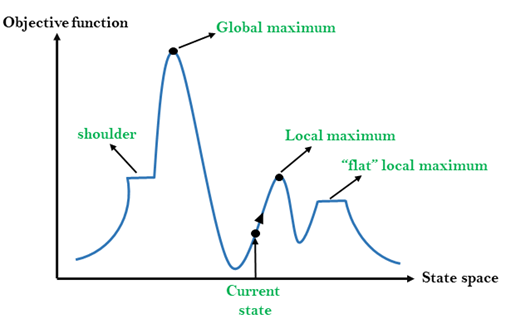
Different regions in the state space landscape:

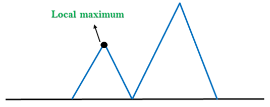
Local Maximum: Local maximum is a state which is better than its neighbor states, but there is also another state which is higher than it.

Global Maximum: Global maximum is the best possible state of state space landscape. It has the highest value of objective function.

Current state: It is a state in a landscape diagram where an agent is currently present.

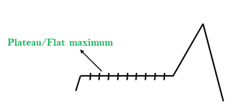
Flat local maximum: It is a flat space in the landscape where all the neighbor states of current states have the same value.

Shoulder: It is a plateau region which has an uphill edge.

Types of Hill Climbing Algorithm:

• Simple hill Climbing:
• Steepest-Ascent hill-climbing:
• Stochastic hill Climbing:

1. Simple Hill Climbing:

Simple hill climbing is the simplest way to implement a hill climbing algorithm. It only evaluates the neighbor node state at a time and selects the first one which optimizes current cost and set it as a current state. It only checks it's one successor state, and if it finds better than the current state, then move else be in the same state. This algorithm has the following features:

• Less time consuming
• Less optimal solution and the solution is not guaranteed

Algorithm for Simple Hill Climbing:

• Step 1: Evaluate the initial state, if it is goal state then return success and Stop.
• Step 2: Loop Until a solution is found or there is no new operator left to apply.
• Step 3: Select and apply an operator to the current state.
• Step 4: Check new state:
  1. If it is goal state, then return success and quit.
  2. Else if it is better than the current state then assign new state as a current state.
  3. Else if not better than the current state, then return to step2.
• Step 5: Exit.

2. Steepest-Ascent hill climbing:

The steepest-Ascent algorithm is a variation of simple hill climbing algorithm. This algorithm examines all the neighboring nodes of the current state and selects one neighbor node which is closest to the goal state. This algorithm consumes more time as it searches for multiple neighbors

Algorithm for Steepest-Ascent hill climbing:

• Step 1: Evaluate the initial state, if it is goal state then return success and stop, else make current state as initial state.
• Step 2: Loop until a solution is found or the current state does not change.
  1. Let SUCC be a state such that any successor of the current state will be better than it.
  2. For each operator that applies to the current state:
     1. Apply the new operator and generate a new state.
     2. Evaluate the new state.
     3. If it is goal state, then return it and quit, else compare it to the SUCC.
     4. If it is better than SUCC, then set new state as SUCC.
     5. If the SUCC is better than the current state, then set current state to SUCC.
• Step 5: Exit.

3. Stochastic hill climbing:

Stochastic hill climbing does not examine for all its neighbor before moving. Rather, this search algorithm selects one neighbor node at random and decides whether to choose it as a current state or examine another state.

Problems in Hill Climbing Algorithm:

1. Local Maximum: A local maximum is a peak state in the landscape which is better than each of its neighboring states, but there is another state also present which is higher than the local maximum. 

Solution: Backtracking technique can be a solution of the local maximum in state space landscape. Create a list of the promising path so that the algorithm can backtrack the search space and explore other paths as well.

2. Plateau: A plateau is the flat area of the search space in which all the neighbor states of the current state contains the same value, because of this algorithm does not find any best direction to move. A hill-climbing search might be lost in the plateau area.

Solution: The solution for the plateau is to take big steps or very little steps while searching, to solve the problem. Randomly select a state which is far away from the current state so it is possible that the algorithm could find non-plateau region.

3. Ridges: A ridge is a special form of the local maximum. It has an area which is higher than its surrounding areas, but itself has a slope, and cannot be reached in a single move.

Solution: With the use of bidirectional search, or by moving in different directions, we can improve this problem.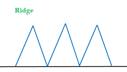

Simulated Annealing:

A hill-climbing algorithm which never makes a move towards a lower value guaranteed to be incomplete because it can get stuck on a local maximum. And if algorithm applies a random walk, by moving a successor, then it may complete but not efficient. Simulated Annealing is an algorithm which yields both efficiency and completeness.

In mechanical term Annealing is a process of hardening a metal or glass to a high temperature then cooling gradually, so this allows the metal to reach a low-energy crystalline state. The same process is used in simulated annealing in which the algorithm picks a random move, instead of picking the best move. If the random move improves the state, then it follows the same path. Otherwise, the algorithm follows the path which has a probability of less than 1 or it moves downhill and chooses another path.

Travelling Sales Person Problem

The traveling salesman problems abide by a salesman and a set of cities. The salesman has to visit every one of the cities starting from a certain one (e.g., the hometown) and to return to the same city. The challenge of the problem is that the traveling salesman needs to minimize the total length of the trip.

Suppose the cities are x₁ x₂..... x_n where cost c_ij denotes the cost of travelling from city x_i to x_j. The travelling salesperson problem is to find a route starting and ending at x₁ that will take in all cities with the minimum cost.

Example: A newspaper agent daily drops the newspaper to the area assigned in such a manner that he has to cover all the houses in the respective area with minimum travel cost. Compute the minimum travel cost.

The area assigned to the agent where he has to drop the newspaper is shown in fig:

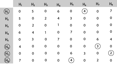
Solution: The cost- adjacency matrix of graph G is as follows:

cost_ij =

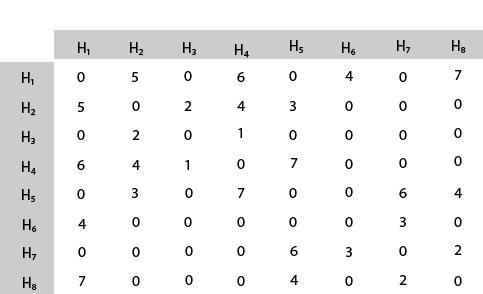
The tour starts from area H₁ and then select the minimum cost area reachable from H₁.

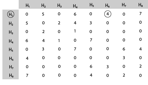
Mark area H₆ because it is the minimum cost area reachable from H₁ and then select minimum cost area reachable from H₆.

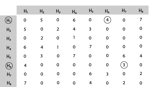
Mark area H₇ because it is the minimum cost area reachable from H₆ and then select minimum cost area reachable from H₇.

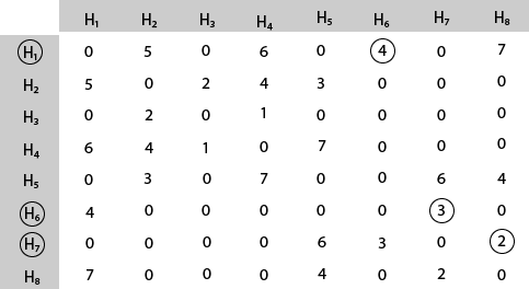
Mark area H₈ because it is the minimum cost area reachable from H₈.

Mark area H₅ because it is the minimum cost area reachable from H₅.

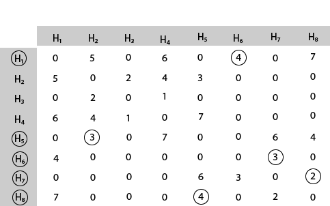
Mark area H₂ because it is the minimum cost area reachable from H₂.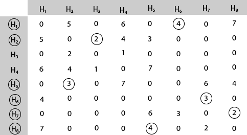

Mark area H₃ because it is the minimum cost area reachable from H₃.

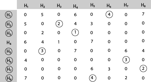
Mark area H₄ and then select the minimum cost area reachable from H₄ it is H₁.So, using the greedy strategy, we get the following.

4    3    2    4    3    2   1    6
H1 → H6 → H7 → H8 → H5 → H2 → H3 → H4 → H1.

Thus the minimum travel cost = 4 + 3 + 2 + 4 + 3 + 2 + 1 + 6 = 25

Videos :

 

Thanks for reading the article. If you have any doubt or just wants to talk Data Science, write it in the comments below.